Finite Element Analysis

I've been writing FEA codes since my junior undergraduate year. Since then I have develop a wide range of 2D/3D finite element codes for both steady state and transient problems. Some details are given below.

2D/3D Elastostatics/Heat Conduction/Thermoelasticity

I began work on this code when I started my Master's degree program in 1995. The main focus was to produce a code that could do thermoelastic stress analysis of internally cooled turbine blades very quickly. At that time our group was heavily involved in a project concerning the optimization of internal coolant passages for turbine blades. Since the optimization code might require hundreds or even thousands of analysis calls, it was important that each analysis take the minimum amount of computation time possible. I spent a lot of time developing iterative sparse equation solvers as a replacement for the direct factorizations used in many FEA codes. Use of such iterative methods resulted in a significant improvement in speed and much lower core memory usage. Currently, the 3D stress/thermal analysis of a realistic turbine blade with passages takes less than one minute on a Pentium II PC.

Some features of the code:

Sparse solvers:

Preconditioned Krylov subspace methods(GMRES, CG, CGS, BiCGSTAB)
ILU and multilevel preconditioners
LU Decomposition(direct solver)
Cholesky Decomposition(VSS from NASA Langley)
Multigrid(2D) for nested and solution adapted grids
Uses of the Enthalpy method to handle phase change for simulation of melting/freezing
Can handle unsteady heat conduction problems with nonlinear material properties
High speed, automatic, suitable for optimization
Objected-oriented, written in C++/C/FORTRAN
Triangular and Tetrahedral elements with a choice of linear or quadratic basis functions
Element stiffness matrices integrated analytically

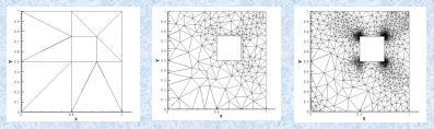
The 2D version of my code uses adaptive mesh refinement. Here's an example for heat conduction:

Code Performance
11,000 DOF 3D Turbine Blade (Static): less than 1 min. on Pentium 200, around 15 sec. On SGI R10000
66,000 DOF 3D Turbine Blade (Static): approx. 10 min. on SGI R10000
11,000 DOF 3D Turbine Blade (Dynamic): approx. 5 min. for 100 time steps on Pentium 200

Click on the images below to see a larger picture

Radial normal stresses for steel internally cooled turbine blade at 500 RPM

Deformations(x200) for internally cooled steel turbine blade spinning at 500 RPM

Temperature distribution

Thermally induced stresses

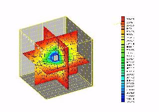
Temperature distribution on two planar slices of a cube with a cavity in the center

3D Structural Dynamics

I also wrote an FEA code for 3D structural dynamics. Currently, this code has not been used in any projects. It may eventually be used for aeroelastic simulations of turbomachinery blades. Click on the links below to see some animation of structural dynamics results produced with my code.

Vibrating Beam
Blade
Blade2
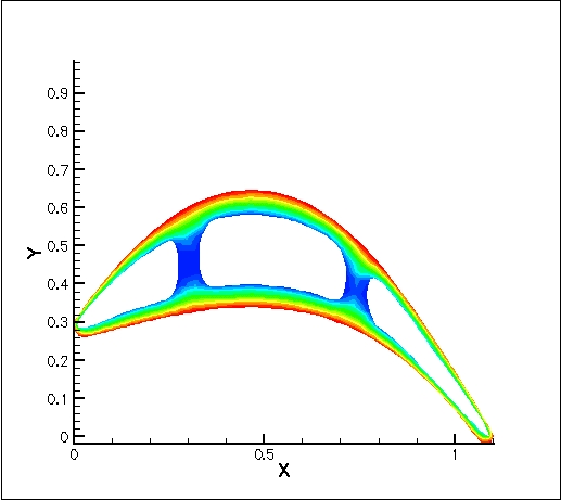
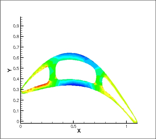
Blade with Passages
Blade with Passages 2

Inverse detection of boundary conditions in 2D thermoelasticity

I developed a finite element algorithm for the inverse detection of unknown boundary conditions for Laplace and Navier equations. I also implemented this algorithm in my 2D thermoelastic finite element code. Below is an example of a forward and inverse heat conduction analysis of an annual region with 16 internal circular cavities. In the well-posed or forward problem, a Dirichlet boundary condition is applied on all boundaries. But in the inverse problem, both the Dirichlet and Neumann boundary conditions are applied to outer circular boundary while no boundary conditions are applied to the internal cavities. The inverse FEA code is able to accurate predict the temperature distribution throughout the entire domain, even on the internal boundaries.

Click on the images below to see larger pictures

Well-posed(forward) and inverse analysis

2D Incompressible Navier Stokes/Euler with LSFEM

In the spring of 1999, I began developing several 2D fluid mechanics codes using the Least-Squares Finite Element method (LSFEM).

Advantages of the LSFEM

Can use equal order basis functions for pressure and velocity
No free parameters to tune
can use the first order form of PDE’s
can handle any type of equation and mixed types of equations
Can discretize convection terms without upwinding or explicit artificial dissipation
Clean and robust method
Resulting system of equations is symmetric and positive definite
Simple iterative techniques and multigrid can be used to solve the system of equations
Easy to construct high order approximations via P-methods
rigorous convergence theory exists
strong mathematical background
Always leads to a minimization problem rather than saddle point problem (interpolation function do not need to satisfy LBB condition)

Below is an example of low speed inviscid, rotation flow (Euler equations) over a circle computed with a finite volume based code and with my LSFEM code. One can see that upwinding require by the FVM code for stability creates a noticeable asymmetry in the pressure field. My LSFEM code produces a perfectly symmetric pressure field that matches the analytic solution obtained from potential flow theory.

Click on the image below to see a larger picture

Comparision of FVM and LSFEM for Euler flow around a circle

Below is an example of viscous incompressible flow though a sudden expansion at a Reynolds number of 450.

Click on the image below to see a larger picture

Viscous flow through a sudden expansion for Re=450

2D Magneto-Hydrodynamics with Conjugate Heat Transfer with LSFEM

Recently I have developed a 2D code to simulate magneto-hydrodynamics with conjugate heat transfer.
This code was used to study the effect of an applied magnetic field to the heat transfer (conductive and convective) characteristics of an incompressible, electrically conducting fluid such as seawater.

Conjugate heat transfer problems involve the simultaneous prediction of heat transfer in both the fluid field and the solid wall surrounding the fluid. An example would be a cooled metal pipe carrying a hot liquid.

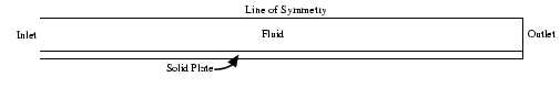In this example, a "horse-shoe" magnet is placed between the X coordinates 7 and 8. In this region, it can be see that the wall temperature changes dramatically, depending on the strength of the magnetic field. It can also be seen that the applied magnetic field generates a complex vortex structure in the flow field. Also, when the magnetic Reynolds number is high (such as when the fluid has a very high coefficient of electrical conductivity), the interaction between the magnetic field and the moving fluid can cause the magnetic field lines to sway in the downstream conditions. This indicates that in MHD problems with high magnetic Reynolds numbers, the Maxwell's equations should always be solved together with the Navier-Stokes equations, either simultaneously or iteratively.

Click on the images below to see a larger picture

Magnetic field lines in the presence of a moving fluid with low electrical conductivity(seawater)	Temperatures along solid/fluid interface for various magnetic field strengths
Vortices induced by the presence of a strong magnetic field	Magnetic field lines in the presence of a highly electrically conductive moving fluid

2D Electro-Magneto-Hydrodynamics with LSFEM

Recently I have developed a 2D code based on LSFEM to simulate electro-magneto-hydrodynamics. This code was used to simulate the pumping of an electrically conducting liquid such as sea water or blood.

In the example shown here,an electric and magnetic field are used pump an electrically conducting incompressible viscous liquid through a channel of height 4 cm and length 40 cm. A a uniform magnetic field of .05 Tesla is applied in the Z direction. A positive electrode is placed at the top of the wall and a negative electrode placed at the bottom of the wall. A potential of 50 Volts applied across the electrodes.A parabolic velocity profile was specified at the inlet and a pressure of 1 Pa was specified at the outlet. The inlet temperature was 311 K and the wall temperature was 300 K

This is a steady state calculation(no time derivatives).

Click on the images below to see a larger picture

Computed electric potential	Computed velocity vectors
Computed static pressure	Computed static temperature

One can see from the above images that the application of a crossed electric and magnetic field results in a pressure increase from the channel inlet to outlet. Without either field, the pressure would decrease from inlet to outlet due to the viscosity of the liquid. The Joule heating of the liquid(due to the flow of electric current through the liquid) can also be seen.

2D Electro-Magneto-Hydrodynamics with p -version LSFEM

Recently I have developed a 2D code based on p-version LSFEM to simulate electro-magneto-hydrodynamics. This code was used to simulate the solidification of silicon crystals with and without an applied magnetic field.

The p-version LSFEM was implemented using hierarchical basis functions based on Jacobi polynomials. The hierarchical basis leads to a linear algebraic system with a natural multilevel structure that is well suited to adaptive enrichment. The sparse linear systems were solved by either direct sparse LU factorization or by iterative methods. Two iterative methods were implemented in the software, one based on a Jacobi preconditioned conjugate gradient and the another based a multigrid-like technique that uses the hierarchy of basis functions instead of a hierarchy of finer grids. The method was implemented in an object-oriented fashion using the C++ programming language. The software has been tested against analytic solutions and experimental data for Navier-Stokes equations and for channel flows through transverse electric and magnetic fields, for shear-driven cavity flows, buoyancy-driven cavity flows, and flow over a backward-facing step.

In the example shown here, a crucible for the production of silicon crystals is simulated with and without an applied uniform magnetic field in the vertical direction. The magnetic field strength is 1 Tesla.

This is a steady state calculation(no time derivatives).

Click on the images below to see a larger picture

Computational mesh

Computed streamlines with no magnetic field and microgravity (1% of full gravity)

Computed streamlines with no magnetic field and full gravity

Computed streamlines with magnetic field and full gravity

One can see from the above images that the application of uniform magnetic field in the vertical direction can significantly alter the flow field melt region of the crucible.

The computational results indicate significantly different flow-field patterns and thermal fields in the melt and the accrued solid in the cases of full gravity, reduced gravity, and an applied uniform magnetic field. Although the magnetic field significantly reduces the velocity of the flow within the melt, the crystal may still be slightly contaminated.